Backpropagation

Modern neural networks often consist of multiple layers and a large number of parameters, sometimes reaching millions. The central challenge in training such networks is determining how to efficiently update these parameters so that the model’s predictions improve over time. This learning process is achieved through an algorithm known as backpropagation, which systematically computes gradients of the loss function with respect to each parameter in the network.

Build Intuition of Chain Rule of Calculus

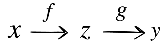
Consider we have a function $g(f(x))$

Chain Rule of Calculus (scaler case):

Consider,

$z=f(x)=x^2$

$y=g(z)=e^z=e^{x^2}$

We can calculate $\frac{dy}{dz}$ and $\frac{dz}{dx}$ easily.

\frac{dy}{dz}=e^z, \;\;\;\;\; \frac{dz}{dx}=2x

But how would you calculate $\frac{dy}{dx}$ here? We have to apply chain rule here.

\frac{dy}{dx}=\frac{dy}{dz}.\frac{dz}{dx}

=e^z.2x=e^{x^2}.2x

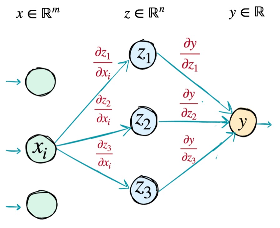
Chain Rule of Calculus (vector case):

Here each $z_i$ is a function of $x = \begin{bmatrix} x_1 \\ x_2 \\ .\\ .\\ x_m \end{bmatrix}$ and $y$ is a function of $z = \begin{bmatrix} z_1 \\ z_2 \\ .\\ .\\ z_n \end{bmatrix}$ . So how do we calculate $\frac{\partial y}{\partial x_i}$ for any $x_i$ ?

Now to understand it simply, earlier for scaler case we just had only one path from $x$ to $z$ to $y$ ( $x \to z \to y$ ). Now for vector case here we have three paths from $x_i$ to $y$ (considering $n=3$ ). So we have to apply chain rule in all the three paths and take the summation.

\frac{\partial y}{\partial x_i}=\frac{\partial y}{\partial z_1}.\frac{\partial z_1}{\partial x_i}+ \frac{\partial y}{\partial z_2}.\frac{\partial z_2}{\partial x_i}+ \frac{\partial y}{\partial z_3}.\frac{\partial z_3}{\partial x_i}

Basically,

\frac{\partial y}{\partial x_i}=\sum_{j=1}^n \frac{\partial y}{\partial z_j}.\frac{\partial z_j}{\partial x_i}

What Is Our Target Here?

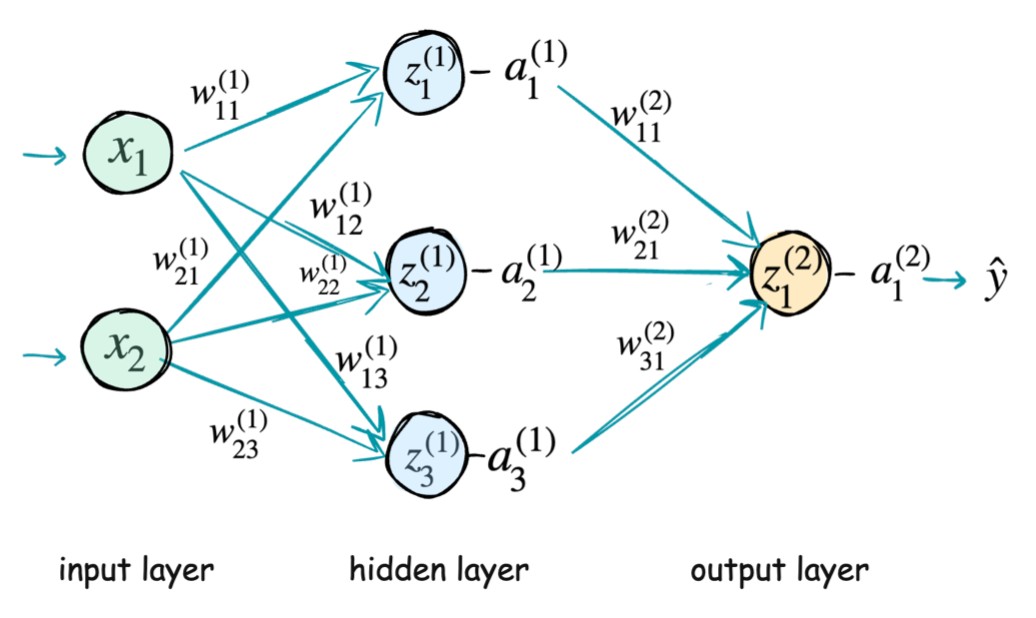
We want to train the model, that means we came up with the neural network model structure but we want to find the optimized weight parameters here. Weight parameters are named as $w_{ij}^{(l)}$ and it means the weight from node $i$ from previous layer to node $j$ in the current layer and current layer is $l$ (starting from the first hidden layer).

How do we find the optimizer proper weights? We run Gradient Descent algorithm and weight parameters are updated in each iteration.

w^{t+1} = w^t - \alpha \frac{\partial E}{\partial w^t}

$w^t$ contains all the weight parameters $w_{ij}^{(l)}$ .

So at each iteration, our target is to find $\frac{\partial E}{\partial w_{ij}^{(l)}}$ for all the weight parameters.

What is $E$ here? $E$ is the Error or Loss we found comparing the actual output $(y)$ and predicted output $(\hat{y})$ .

Loss/Error Functions

There are various types of Loss/Error functions depending on the task we want to perform. Here are few examples..

Mean Square Error(MSE)

Used mostly in linear regression problems.

E= \frac{1}{n} \sum_{i=1}^n {(y_i-\hat{y_i})}^2

Root Mean Square Error(RMSE)

Just taking square root of Mean Square Error

E= \sqrt{\frac{1}{n} \sum_{i=1}^n {(y_i-\hat{y_i})}^2}

Mean Absolute Error (MAE)

Sum of absolute differences between actual and predicted outputs

E= \frac{1}{n} \sum_{i=1}^n {|y_i-\hat{y_i}|}

Binary Cross-Entropy

Used in binary classification

E= -y \; log(\hat{y}) - (1-y)log (1-\hat{y})

Categorical Cross-Entropy

Used in multi-class classification when outputs are represented as one-hot encoding format and there are $K$ classes

E= - \sum_{k=1}^K y_k log(\hat{y_k})

Sparse Categorical Cross-Entropy

Used in multi-class classification when outputs are represented with class indices $(1,2,.. K)$ , $y$ is the correct class index and $\hat{y}_y$ is the predicted probability of correct class $y$

E = - log(\hat{y}_y)

Backward Propagation of Errors

Now we will see how we calculate the gradient of the error (or loss) with respect to all the weights. We start from the output layer and move back towards the input layer.

We are considering binary cross entropy loss for our discussion here.

E= -y \; log(\hat{y}) - (1-y)log (1-\hat{y})

Output Layer Gradients

\frac{\delta E}{\delta \hat{y}}= -\frac{y}{\hat{y}} - \frac{1-y}{1-\hat{y}}(-1)=-\frac{y}{\hat{y}} - \frac{y-1}{1-\hat{y}}

As $a_1^{(2)}=\hat{y}$ ,

\frac{\delta E}{\delta a_1^{(2)}}= \frac{\delta E}{\delta \hat{y}}

Now assume $a_1^{(2)}$ uses sigmoid activation function or $a_1^{(2)}=\sigma(z_1^{(2)})$ .

We already know how to calculate the derivative of sigmoid [ $\sigma ^{'} (a) = \sigma (a)(1- \sigma(a))$ ]

\frac{\delta a_1^{(2)}}{\delta z_1^{(2)}}=\sigma(z_1^{(2)})(1-\sigma(z_1^{(2)}))

Now how do we calculate $\frac{\delta E}{\delta z_1^{(2)}}$ ? We have to apply chain rule.

\frac{\delta E}{\delta z_1^{(2)}}= \frac{\delta E}{\delta a_1^{(2)}}.\frac{\delta a_1^{(2)}}{\delta z_1^{(2)}}=\frac{\delta E}{\delta \hat{y}}.\frac{\delta a_1^{(2)}}{\delta z_1^{(2)}}

Second Layer Gradients

Here $z_1^{(2)}$ is the linear weighted combination of previous layer neurons. Also, biases ( like $w_{01}^{(2)}$ ) are not shown in the diagram so you just assume they are there :)

z_1^{(2)}=w_{01}^{(2)}+w_{11}^{(2)}a_1^{(1)}+w_{21}^{(2)}a_2^{(1)}+w_{31}^{(2)}a_3^{(1)}

Hence,

\frac{\delta z_1^{(2)}}{\delta w_{11}^{(2)}}=a_1^{(1)}, \; \; \frac{\delta z_1^{(2)}}{\delta w_{21}^{(2)}}=a_2^{(1)} \;\; \frac{\delta z_1^{(2)}}{\delta w_{31}^{(2)}}=a_3^{(1)}

So Gradients with respect to second layer weights can be calculated using chain rule.

\frac{\delta E}{\delta w_{11}^{(2)}}= \frac{\delta E}{\delta z_1^{(2)}}.\frac{\delta z_1^{(2)}}{\delta w_{11}^{(2)}}

\frac{\delta E}{\delta w_{21}^{(2)}}= \frac{\delta E}{\delta z_1^{(2)}}.\frac{\delta z_1^{(2)}}{\delta w_{21}^{(2)}}

\frac{\delta E}{\delta w_{31}^{(2)}}= \frac{\delta E}{\delta z_1^{(2)}}.\frac{\delta z_1^{(2)}}{\delta w_{31}^{(2)}}

First Layer Gradients

z_1^{(2)}=w_{01}^{(2)}+w_{11}^{(2)}a_1^{(1)}+w_{21}^{(2)}a_2^{(1)}+w_{31}^{(2)}a_3^{(1)}

What is $\frac{\partial z_1^{(2)}}{\partial a_1^{(1)}}$ ?

\frac{\partial z_1^{(2)}}{\partial a_1^{(1)}}=w_{11}^{(2)}

What is $\frac{\partial a_1^{(1)}}{\partial z_1^{(1)}}$ ? It depends on the activation function used in $a_1^{(1)}$ .

Mostly for hidden layers we use Relu as activation function $(f(x)=max(0, x))$ . Derivative of relu is 1 if $x > 0$ , 0 if $x < 0$ and it is undefined at 0.

$z_1^{(1)}$ is a weighted linear combination of first layer weights.

z_1^{(1)}=w_{01}^{(1)}+w_{11}^{(1)}x_1+w_{21}^{(1)}x_2

By using chain rule we will calculate $\frac{\partial E}{\delta w_{11}^{(1)}}$ and other gradients with respect to first layer weights in the same way.

\frac{\partial E}{\delta w_{11}^{(1)}}= \frac{\partial E}{\partial z_1^{(2)}}. \frac{\partial z_1^{(2)}}{\partial a_1^{(1)}}.\frac{\partial a_1^{(1)}}{\partial z_1^{(1)}}.\frac{\partial z_1^{(1)}}{\partial w_{11}^{(1)}}

Visualize Error Backpropagation

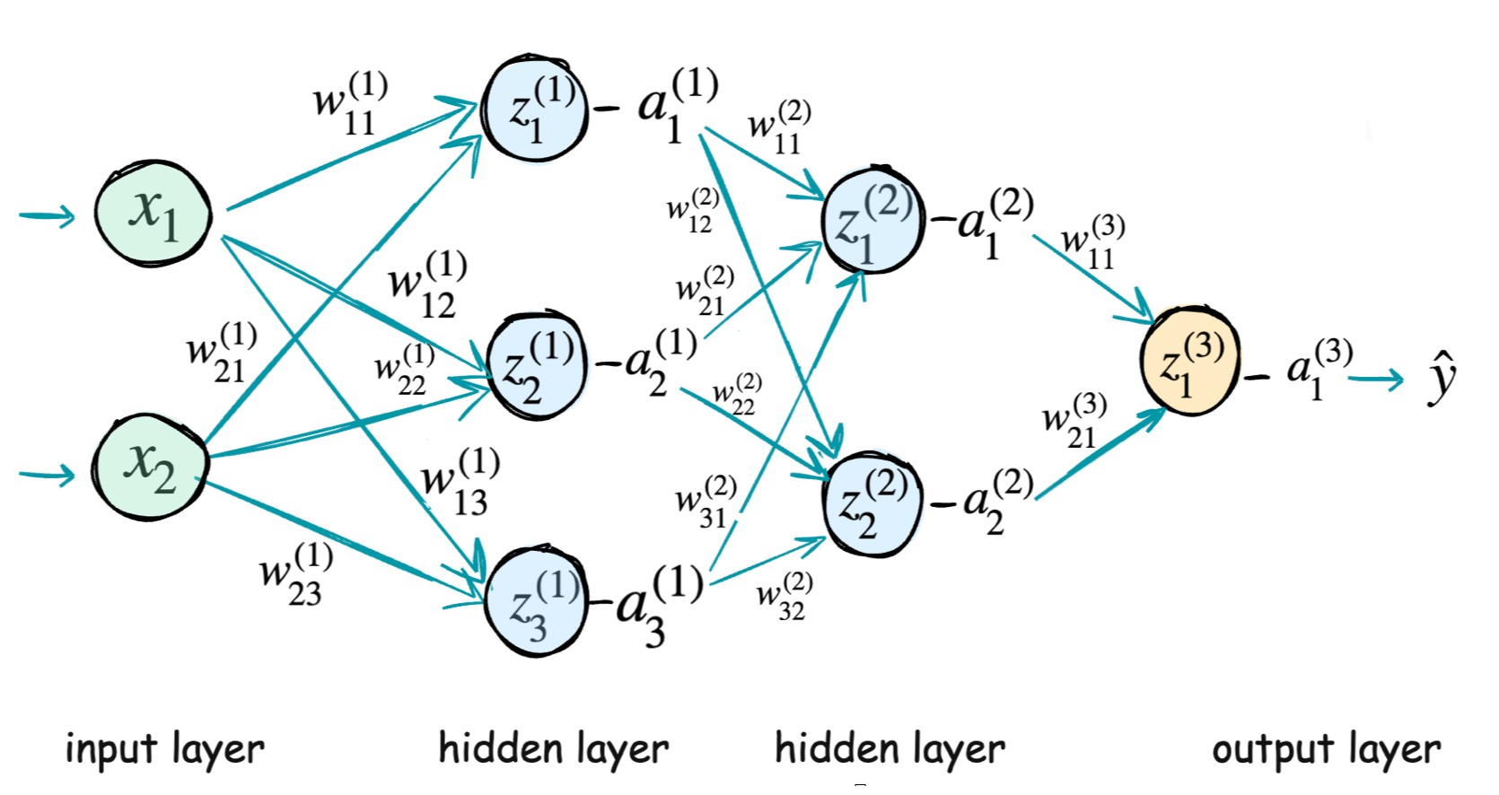
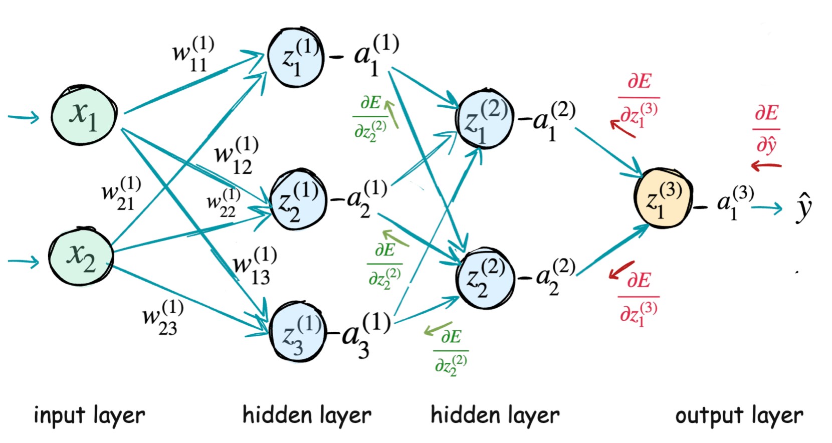
Here we are considering a different network with two hidden layers and we will see how error gradients are flowing backward from output layer to input layers.

Here $z_1^{(3)}$ is a combination of $a_1^{(2)}$ and $a_2^{(2)}$ . So $\frac{\partial E}{\partial z_1^{(3)}}$ will flow in both the path as shown in the image.

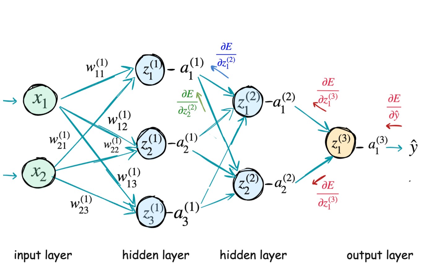
$\frac{\partial E}{\partial z_1^{(2)}}$ will flow backward to three paths corresponding to $a_1^{(1)}$ , $a_2^{(1)}$ and $a_3^{(1)}$ . Similarly, $\frac{\partial E}{\partial z_2^{(2)}}$ will also flow backward to three paths corresponding to $a_1^{(1)}$ , $a_2^{(1)}$ and $a_3^{(1)}$ .

How do you calculate $\frac{\partial E}{\partial a_1^{(1)}}$ ? $a_1^{(1)}$ is influencing both $z_1^{(2)}$ and $z_2^{(2)}$ . The error $\frac{\partial E}{\partial z_1^{(2)}}$ and $\frac{\partial E}{\partial z_2^{(2)}}$ both backpropagating towards $a_1^{(1)}$ .

So we have to apply vector case for chain rule of calculas..

\frac{\partial E}{\partial a_1^{(1)}}=\frac{\partial E}{\partial z_1^{(2)}}.\frac{\partial z_1^{(2)}}{\partial a_1^{(1)}} +\frac{\partial E}{\partial z_2^{(2)}}.\frac{\partial z_2^{(2)}}{\partial a_1^{(1)}}

$\frac{\partial E}{\partial z_1^{(2)}}$ and $\frac{\partial E}{\partial z_2^{(2)}}$ is already backpropagating towards $a_1^{(1)}$ . We just need to calculate $\frac{\partial z_1^{(2)}}{\partial a_1^{(1)}}$ and $\frac{\partial z_2^{(2)}}{\partial a_1^{(1)}}$ .

z_1^{(2)}=w_{11}^{(2)}a_1^{(1)}+w_{21}^{(2)}a_2^{(1)}+w_{31}^{(2)}a_3^{(1)}

z_2^{(2)}=w_{12}^{(2)}a_1^{(1)}+w_{22}^{(2)}a_2^{(1)}+w_{32}^{(2)}a_3^{(1)}

Hence,

\frac{\partial z_1^{(2)}}{\partial a_1^{(1)}}=w_{11}^{(2)}, \;\; \;\frac{\partial z_1^{(2)}}{\partial a_1^{(1)}}=w_{11}^{(2)}

How Do We Update The Biases?

We will see one small example of how we calculate the gradient w.r.t the biases. Showing just one biad $w_{01}^{(3)}$ while computing $z_1^{(3)}$ .

We will try to calculate $\frac{\partial E}{\partial w_{01}^{(3)}}$ .

z_1^{(3)}=w_{01}^{(3)}+w_{11}^3a_1^{(2)}+w_{21}^{(3)}a_2^{(2)}

Here,

\frac{\partial z_{1}^{(3)}}{\partial w_{01}^{(3)}}=1

Using chain rule,

\frac{\partial E}{\partial w_{01}^{(3)}}=\frac{\partial E}{\partial z_{1}^{(3)}}.\frac{\partial z_{1}^{(3)}}{\partial w_{01}^{(3)}}

Hence,

\frac{\partial E}{\partial w_{01}^{(3)}}=\frac{\partial E}{\partial z_{1}^{(3)}}